Quartile
In statistics, quartiles are a type of quantiles which divide the number of data points into four parts, or quarters, of more-or-less equal size.
The data must be ordered from smallest to largest to compute quartiles; as such, quartiles are a form of order statistic.
This summary is important in statistics because it provides information about both the center and the spread of the data.
Knowing the lower and upper quartile provides information on how big the spread is and if the dataset is skewed toward one side.
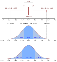
Interquartile range (IQR) is defined as the difference between the 75th and 25th percentiles or Q3 - Q1.
[2] For discrete distributions, there is no universal agreement on selecting the quartile values.
[3] This rule is employed by the TI-83 calculator boxplot and "1-Var Stats" functions.
The values found by this method are also known as "Tukey's hinges";[4] see also midhinge.
The bold number (40) is the median splitting the data set into two halves with equal number of data points.
The bold numbers (36, 39) are used to calculate the median as their average.
As there are an even number of data points, the first three methods all give the same results.
is a real valued random variable, its cumulative distribution function (CDF) is given by
[1] The CDF gives the probability that the random variable
Outliers could be a result from a shift in the location (mean) or in the scale (variability) of the process of interest.
Consequently, as is the basic idea of descriptive statistics, when encountering an outlier, we have to explain this value by further analysis of the cause or origin of the outlier.
In cases of extreme observations, which are not an infrequent occurrence, the typical values must be analyzed.
The Interquartile Range (IQR), defined as the difference between the upper and lower quartiles (
), may be used to characterize the data when there may be extremities that skew the data; the interquartile range is a relatively robust statistic (also sometimes called "resistance") compared to the range and standard deviation.
There is also a mathematical method to check for outliers and determining "fences", upper and lower limits from which to check for outliers.
) as outlined above, then fences are calculated using the following formula: The lower fence is the "lower limit" and the upper fence is the "upper limit" of data, and any data lying outside these defined bounds can be considered an outlier.
It is common for the lower and upper fences along with the outliers to be represented by a boxplot.
For the boxplot shown on the right, only the vertical heights correspond to the visualized data set while horizontal width of the box is irrelevant.
Outliers located outside the fences in a boxplot can be marked as any choice of symbol, such as an "x" or "o".
When spotting an outlier in the data set by calculating the interquartile ranges and boxplot features, it might be easy to mistakenly view it as evidence that the population is non-normal or that the sample is contaminated.
However, this method should not take place of a hypothesis test for determining normality of the population.
The significance of the outliers varies depending on the sample size.
[7] The Excel function QUARTILE.INC(array, quart) provides the desired quartile value for a given array of data, using Method 3 from above.
In the function, array is the dataset of numbers that is being analyzed and quart is any of the following 5 values depending on which quartile is being calculated.
[8] In order to calculate quartiles in Matlab, the function quantile(A,p) can be used.
Where A is the vector of data being analyzed and p is the percentage that relates to the quartiles as stated below.