Integral

Integration was initially used to solve problems in mathematics and physics, such as finding the area under a curve, or determining displacement from velocity.

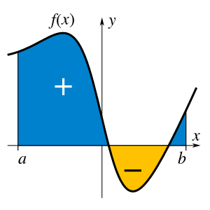
A definite integral computes the signed area of the region in the plane that is bounded by the graph of a given function between two points in the real line.

Although methods of calculating areas and volumes dated from ancient Greek mathematics, the principles of integration were formulated independently by Isaac Newton and Gottfried Wilhelm Leibniz in the late 17th century, who thought of the area under a curve as an infinite sum of rectangles of infinitesimal width.

The first documented systematic technique capable of determining integrals is the method of exhaustion of the ancient Greek astronomer Eudoxus and philosopher Democritus (ca.

[2] A similar method was independently developed in China around the 3rd century AD by Liu Hui, who used it to find the area of the circle.

[3] In the Middle East, Hasan Ibn al-Haytham, Latinized as Alhazen (c. 965 – c. 1040 AD) derived a formula for the sum of fourth powers.

Further steps were made in the early 17th century by Barrow and Torricelli, who provided the first hints of a connection between integration and differentiation.

[10] The major advance in integration came in the 17th century with the independent discovery of the fundamental theorem of calculus by Leibniz and Newton.

This framework eventually became modern calculus, whose notation for integrals is drawn directly from the work of Leibniz.

While Newton and Leibniz provided a systematic approach to integration, their work lacked a degree of rigour.

Bishop Berkeley memorably attacked the vanishing increments used by Newton, calling them "ghosts of departed quantities".

[13] Although all bounded piecewise continuous functions are Riemann-integrable on a bounded interval, subsequently more general functions were considered—particularly in the context of Fourier analysis—to which Riemann's definition does not apply, and Lebesgue formulated a different definition of integral, founded in measure theory (a subfield of real analysis).

[14] He adapted the integral symbol, ∫, from the letter ſ (long s), standing for summa (written as ſumma; Latin for "sum" or "total").

But if it is oval with a rounded bottom, integrals are required to find exact and rigorous values for these quantities.

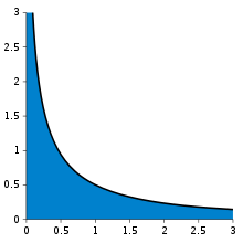
However, when the number of pieces increases to infinity, it will reach a limit which is the exact value of the area sought (in this case, 2/3).

One writes which means 2/3 is the result of a weighted sum of function values, √x, multiplied by the infinitesimal step widths, denoted by dx, on the interval [0, 1].

I take the bills and coins out of my pocket and give them to the creditor in the order I find them until I have reached the total sum.

After I have taken all the money out of my pocket I order the bills and coins according to identical values and then I pay the several heaps one after the other to the creditor.

Using the "partitioning the range of f " philosophy, the integral of a non-negative function f : R → R should be the sum over t of the areas between a thin horizontal strip between y = t and y = t + dt.

Linearity, together with some natural continuity properties and normalization for a certain class of "simple" functions, may be used to give an alternative definition of the integral.

Here the basic differentials dx, dy, dz measure infinitesimal oriented lengths parallel to the three coordinate axes.

In the case of a simple disc created by rotating a curve about the x-axis, the radius is given by f(x), and its height is the differential dx.

The most basic technique for computing definite integrals of one real variable is based on the fundamental theorem of calculus.

More recently a new approach has emerged, using D-finite functions, which are the solutions of linear differential equations with polynomial coefficients.

[54] The method of brackets is a generalization of Ramanujan's master theorem that can be applied to a wide range of univariate and multivariate integrals.

A set of rules are applied to the coefficients and exponential terms of the integrand's power series expansion to determine the integral.

The trapezoidal rule weights the first and last values by one half, then multiplies by the step width to obtain a better approximation.

[58] Higher degree Newton–Cotes approximations can be more accurate, but they require more function evaluations, and they can suffer from numerical inaccuracy due to Runge's phenomenon.

Romberg's method halves the step widths incrementally, giving trapezoid approximations denoted by T(h0), T(h1), and so on, where hk+1 is half of hk.

Kempf, Jackson and Morales demonstrated mathematical relations that allow an integral to be calculated by means of differentiation.