Coefficient of determination
This can arise when the predictions that are being compared to the corresponding outcomes have not been derived from a model-fitting procedure using those data.
Even if a model-fitting procedure has been used, R2 may still be negative, for example when linear regression is conducted without including an intercept,[5] or when a non-linear function is used to fit the data.
The coefficient of determination can be more intuitively informative than MAE, MAPE, MSE, and RMSE in regression analysis evaluation, as the former can be expressed as a percentage, whereas the latter measures have arbitrary ranges.
[7] When evaluating the goodness-of-fit of simulated (Ypred) versus measured (Yobs) values, it is not appropriate to base this on the R2 of the linear regression (i.e., Yobs= m·Ypred + b).
then the variability of the data set can be measured with two sums of squares formulas: The most general definition of the coefficient of determination is
This partition of the sum of squares holds for instance when the model values ƒi have been obtained by linear regression.
This set of conditions is an important one and it has a number of implications for the properties of the fitted residuals and the modelled values.
In particular, under these conditions: In linear least squares multiple regression (with fitted intercept and slope), R2 equals
In a linear least squares regression with a single explanator (with fitted intercept and slope), this is also equal to
[citation needed] According to Everitt,[10] this usage is specifically the definition of the term "coefficient of determination": the square of the correlation between two (general) variables.
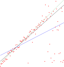
This illustrates a drawback to one possible use of R2, where one might keep adding variables (kitchen sink regression) to increase the R2 value.
Consider a linear model with more than a single explanatory variable, of the form where, for the ith case,
The optimal value of the objective is weakly smaller as more explanatory variables are added and hence additional columns of
When the extra variable is included, the data always have the option of giving it an estimated coefficient of zero, leaving the predicted values and the R2 unchanged.
[14] A simple case to be considered first: This equation describes the ordinary least squares regression model with one regressor.
) is an attempt to account for the phenomenon of the R2 automatically increasing when extra explanatory variables are added to the model.
Inserting the degrees of freedom and using the definition of R2, it can be rewritten as: where p is the total number of explanatory variables in the model (excluding the intercept), and n is the sample size.
If a set of explanatory variables with a predetermined hierarchy of importance are introduced into a regression one at a time, with the adjusted R2 computed each time, the level at which adjusted R2 reaches a maximum, and decreases afterward, would be the regression with the ideal combination of having the best fit without excess/unnecessary terms.
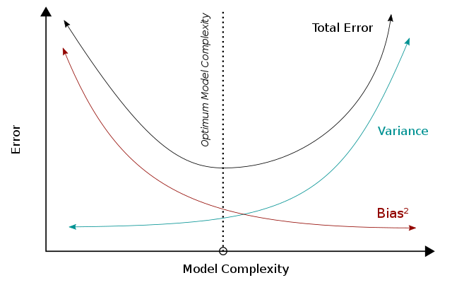
When the model becomes more complex, the variance will increase whereas the square of bias will decrease, and these two metrices add up to be the total error.
Combining these two trends, the bias-variance tradeoff describes a relationship between the performance of the model and its complexity, which is shown as a u-shape curve on the right.
A high R2 indicates a lower bias error because the model can better explain the change of Y with predictors.
For this reason, we make fewer (erroneous) assumptions, and this results in a lower bias error.
Based on bias-variance tradeoff, a higher complexity will lead to a decrease in bias and a better performance (below the optimal line).
In R2, the term (1 − R2) will be lower with high complexity and resulting in a higher R2, consistently indicating a better performance.
Based on bias-variance tradeoff, a higher model complexity (beyond the optimal line) leads to increasing errors and a worse performance.
The calculation for the partial R2 is relatively straightforward after estimating two models and generating the ANOVA tables for them.
The calculation for the partial R2 is which is analogous to the usual coefficient of determination: As explained above, model selection heuristics such as the adjusted R2 criterion and the F-test examine whether the total R2 sufficiently increases to determine if a new regressor should be added to the model.
[24] As Hoornweg (2018) shows, several shrinkage estimators – such as Bayesian linear regression, ridge regression, and the (adaptive) lasso – make use of this decomposition of R2 when they gradually shrink parameters from the unrestricted OLS solutions towards the hypothesized values.
Let us first define the linear regression model as It is assumed that the matrix X is standardized with Z-scores and that the column vector
To deal with such uncertainties, several shrinkage estimators implicitly take a weighted average of the diagonal elements of

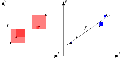

The better the linear regression (on the right) fits the data in comparison to the simple average (on the left graph), the closer the value of R 2 is to 1. The areas of the blue squares represent the squared residuals with respect to the linear regression. The areas of the red squares represent the squared residuals with respect to the average value.