Correlation
Although in the broadest sense, "correlation" may indicate any type of association, in statistics it usually refers to the degree to which a pair of variables are linearly related.
In this example, there is a causal relationship, because extreme weather causes people to use more electricity for heating or cooling.
Formally, random variables are dependent if they do not satisfy a mathematical property of probabilistic independence.
However, when used in a technical sense, correlation refers to any of several specific types of mathematical relationship between the conditional expectation of one variable given the other is not constant as the conditioning variable changes; broadly correlation in this specific sense is used when
It is obtained by taking the ratio of the covariance of the two variables in question of our numerical dataset, normalized to the square root of their variances.
Mathematically, one simply divides the covariance of the two variables by the product of their standard deviations.
Karl Pearson developed the coefficient from a similar but slightly different idea by Francis Galton.
[4] A Pearson product-moment correlation coefficient attempts to establish a line of best fit through a dataset of two variables by essentially laying out the expected values and the resulting Pearson's correlation coefficient indicates how far away the actual dataset is from the expected values.
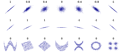
It is a corollary of the Cauchy–Schwarz inequality that the absolute value of the Pearson correlation coefficient is not bigger than 1.
The correlation coefficient is +1 in the case of a perfect direct (increasing) linear relationship (correlation), −1 in the case of a perfect inverse (decreasing) linear relationship (anti-correlation),[5] and some value in the open interval
However, because the correlation coefficient detects only linear dependencies between two variables, the converse is not necessarily true.
For this joint distribution, the marginal distributions are: This yields the following expectations and variances: Therefore: Rank correlation coefficients, such as Spearman's rank correlation coefficient and Kendall's rank correlation coefficient (τ) measure the extent to which, as one variable increases, the other variable tends to increase, without requiring that increase to be represented by a linear relationship.
The information given by a correlation coefficient is not enough to define the dependence structure between random variables.
In the case of elliptical distributions it characterizes the (hyper-)ellipses of equal density; however, it does not completely characterize the dependence structure (for example, a multivariate t-distribution's degrees of freedom determine the level of tail dependence).
For continuous variables, multiple alternative measures of dependence were introduced to address the deficiency of Pearson's correlation that it can be zero for dependent random variables (see [9] and reference references therein for an overview).
One important disadvantage of the alternative, more general measures is that, when used to test whether two variables are associated, they tend to have lower power compared to Pearson's correlation when the data follow a multivariate normal distribution.
[14] For two binary variables, the odds ratio measures their dependence, and takes range non-negative numbers, possibly infinity:
That is, if we are analyzing the relationship between X and Y, most correlation measures are unaffected by transforming X to a + bX and Y to c + dY, where a, b, c, and d are constants (b and d being positive).
Sample-based statistics intended to estimate population measures of dependence may or may not have desirable statistical properties such as being unbiased, or asymptotically consistent, based on the spatial structure of the population from which the data were sampled.
In 2002, Higham[17] formalized the notion of nearness using the Frobenius norm and provided a method for computing the nearest correlation matrix using the Dykstra's projection algorithm, of which an implementation is available as an online Web API.
[18] This sparked interest in the subject, with new theoretical (e.g., computing the nearest correlation matrix with factor structure[19]) and numerical (e.g. usage the Newton's method for computing the nearest correlation matrix[20]) results obtained in the subsequent years.
[22] This dictum should not be taken to mean that correlations cannot indicate the potential existence of causal relations.
Consequently, a correlation between two variables is not a sufficient condition to establish a causal relationship (in either direction).
The second one (top right) is not distributed normally; while an obvious relationship between the two variables can be observed, it is not linear.
In the third case (bottom left), the linear relationship is perfect, except for one outlier which exerts enough influence to lower the correlation coefficient from 1 to 0.816.
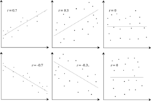
These examples indicate that the correlation coefficient, as a summary statistic, cannot replace visual examination of the data.
The examples are sometimes said to demonstrate that the Pearson correlation assumes that the data follow a normal distribution, but this is only partially correct.
However, the Pearson correlation coefficient (taken together with the sample mean and variance) is only a sufficient statistic if the data is drawn from a multivariate normal distribution.
As a result, the Pearson correlation coefficient fully characterizes the relationship between variables if and only if the data are drawn from a multivariate normal distribution.
of random variables follows a bivariate normal distribution, the conditional mean