Linear regression
Often these n equations are stacked together and written in matrix notation as where Fitting a linear model to a given data set usually requires estimating the regression coefficients
Consider a situation where a small ball is being tossed up in the air and then we measure its heights of ascent hi at various moments in time ti.
Physics tells us that, ignoring the drag, the relationship can be modeled as where β1 determines the initial velocity of the ball, β2 is proportional to the standard gravity, and εi is due to measurement errors.
Numerous extensions have been developed that allow each of these assumptions to be relaxed (i.e. reduced to a weaker form), and in some cases eliminated entirely.
Generally these extensions make the estimation procedure more complex and time-consuming, and may also require more data in order to produce an equally precise model.
Alternatively, the expression "held fixed" can refer to a selection that takes place in the context of data analysis.
The notion of a "unique effect" is appealing when studying a complex system where multiple interrelated components influence the response variable.
In some cases, it can literally be interpreted as the causal effect of an intervention that is linked to the value of a predictor variable.
[9] Numerous extensions of linear regression have been developed, which allow some or all of the assumptions underlying the basic model to be relaxed.
The general linear model considers the situation when the response variable is not a scalar (for each observation) but a vector, yi.
This is used, for example: Generalized linear models allow for an arbitrary link function, g, that relates the mean of the response variable(s) to the predictors:
Under certain conditions, simply applying OLS to data from a single-index model will consistently estimate β up to a proportionality constant.
Group effects provide a means to study the collective impact of strongly correlated predictor variables in linear regression models.
Furthermore, when the sample size is not large, none of their parameters can be accurately estimated by the least squares regression due to the multicollinearity problem.
With strong positive correlations and in standardized units, variables in the group are approximately equal, so they are likely to increase at the same time and in similar amount.
strongly correlated predictor variables in an APC arrangement in the standardized model, group effects whose weight vectors
, and (3) characterizing the region of the predictor variable space over which predictions by the least squares estimated model are accurate.
The combination of swept or unswept matrices provides an alternative method for estimating linear regression models.
These methods differ in computational simplicity of algorithms, presence of a closed-form solution, robustness with respect to heavy-tailed distributions, and theoretical assumptions needed to validate desirable statistical properties such as consistency and asymptotic efficiency.
In the least-squares setting, the optimum parameter vector is defined as such that minimizes the sum of mean squared loss: Now putting the independent and dependent variables in matrices
is a random variable that follows a Gaussian distribution, where the standard deviation is fixed and the mean is a linear combination of
[21] Linear regression is widely used in biological, behavioral and social sciences to describe possible relationships between variables.
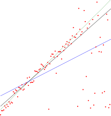
A trend line could simply be drawn by eye through a set of data points, but more properly their position and slope is calculated using statistical techniques like linear regression.
Trend lines are often used to argue that a particular action or event (such as training, or an advertising campaign) caused observed changes at a point in time.
Early evidence relating tobacco smoking to mortality and morbidity came from observational studies employing regression analysis.
For this reason, randomized controlled trials are often able to generate more compelling evidence of causal relationships than can be obtained using regression analyses of observational data.
The capital asset pricing model uses linear regression as well as the concept of beta for analyzing and quantifying the systematic risk of an investment.
[31] One notable example of this application in infectious diseases is the flattening the curve strategy emphasized early in the COVID-19 pandemic, where public health officials dealt with sparse data on infected individuals and sophisticated models of disease transmission to characterize the spread of COVID-19.
[33] Linear regression plays an important role in the subfield of artificial intelligence known as machine learning.
[34] Isaac Newton is credited with inventing "a certain technique known today as linear regression analysis" in his work on equinoxes in 1700, and wrote down the first of the two normal equations of the ordinary least squares method.