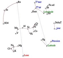
Principal component analysis
These directions (i.e., principal components) constitute an orthonormal basis in which different individual dimensions of the data are linearly uncorrelated.
Factor analysis typically incorporates more domain-specific assumptions about the underlying structure and solves eigenvectors of a slightly different matrix.
[7][8][9][6] PCA was invented in 1901 by Karl Pearson,[10] as an analogue of the principal axis theorem in mechanics; it was later independently developed and named by Harold Hotelling in the 1930s.
Columns of W multiplied by the square root of corresponding eigenvalues, that is, eigenvectors scaled up by the variances, are called loadings in PCA or in Factor analysis.
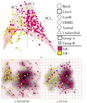
Keeping only the first L principal components, produced by using only the first L eigenvectors, gives the truncated transformation where the matrix TL now has n rows but only L columns.
Similarly, in regression analysis, the larger the number of explanatory variables allowed, the greater is the chance of overfitting the model, producing conclusions that fail to generalise to other datasets.
Each eigenvalue is proportional to the portion of the "variance" (more correctly of the sum of the squared distances of the points from their multidimensional mean) that is associated with each eigenvector.
This advantage, however, comes at the price of greater computational requirements if compared, for example, and when applicable, to the discrete cosine transform, and in particular to the DCT-II which is simply known as the "DCT".
[28][page needed] Researchers at Kansas State University discovered that the sampling error in their experiments impacted the bias of PCA results.
Implemented, for example, in LOBPCG, efficient blocking eliminates the accumulation of the errors, allows using high-level BLAS matrix-matrix product functions, and typically leads to faster convergence, compared to the single-vector one-by-one technique.
The pioneering statistical psychologist Spearman actually developed factor analysis in 1904 for his two-factor theory of intelligence, adding a formal technique to the science of psychometrics.
An extensive literature developed around factorial ecology in urban geography, but the approach went out of fashion after 1980 as being methodologically primitive and having little place in postmodern geographical paradigms.
In 2000, Flood revived the factorial ecology approach to show that principal components analysis actually gave meaningful answers directly, without resorting to factor rotation.
[49] About the same time, the Australian Bureau of Statistics defined distinct indexes of advantage and disadvantage taking the first principal component of sets of key variables that were thought to be important.
The coefficients on items of infrastructure were roughly proportional to the average costs of providing the underlying services, suggesting the Index was actually a measure of effective physical and social investment in the city.
In 1978 Cavalli-Sforza and others pioneered the use of principal components analysis (PCA) to summarise data on variation in human gene frequencies across regions.
In August 2022, the molecular biologist Eran Elhaik published a theoretical paper in Scientific Reports analyzing 12 PCA applications.
For example, the Oxford Internet Survey in 2013 asked 2000 people about their attitudes and beliefs, and from these analysts extracted four principal component dimensions, which they identified as 'escape', 'social networking', 'efficiency', and 'problem creating'.
Valuations here depend on the entire yield curve, comprising numerous highly correlated instruments, and PCA is used to define a set of components or factors that explain rate movements,[59] thereby facilitating the modelling.
[60] Here, for each simulation-sample, the components are stressed, and rates, and in turn option values, are then reconstructed; with VaR calculated, finally, over the entire run.
PCA may also be applied to stress testing,[64] essentially an analysis of a bank's ability to endure a hypothetical adverse economic scenario.
A variant of principal components analysis is used in neuroscience to identify the specific properties of a stimulus that increases a neuron's probability of generating an action potential.
[67] Correspondence analysis (CA) was developed by Jean-Paul Benzécri[68] and is conceptually similar to PCA, but scales the data (which should be non-negative) so that rows and columns are treated equivalently.
In PCA, the contribution of each component is ranked based on the magnitude of its corresponding eigenvalue, which is equivalent to the fractional residual variance (FRV) in analyzing empirical data.
It extends the classic method of principal component analysis (PCA) for the reduction of dimensionality of data by adding sparsity constraint on the input variables.
Several approaches have been proposed, including The methodological and theoretical developments of Sparse PCA as well as its applications in scientific studies were recently reviewed in a survey paper.
Trevor Hastie expanded on this concept by proposing Principal curves[87] as the natural extension for the geometric interpretation of PCA, which explicitly constructs a manifold for data approximation followed by projecting the points onto it.
[7][5] Robust principal component analysis (RPCA) via decomposition in low-rank and sparse matrices is a modification of PCA that works well with respect to grossly corrupted observations.
[97] Discriminant analysis of principal components (DAPC) is a multivariate method used to identify and describe clusters of genetically related individuals.
(more info: adegenet on the web) Directional component analysis (DCA) is a method used in the atmospheric sciences for analysing multivariate datasets.


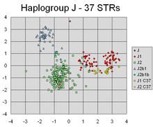
PCA has successfully found linear combinations of the markers that separate out different clusters corresponding to different lines of individuals' Y-chromosomal genetic descent.